About Lightweight CNNs: The MobileNet Series

Lightweight Networks

The progress of deep learning began alongside the progress of hardware. Without a sufficiently capable CPU or GPU, we cannot fully use a network with strong inference performance.

We cannot run deep learning forever on a heavy server machine, however, so simplifying and reducing the size of neural networks is essential.

The purpose of a lightweight network can therefore be divided into two goals.

1. Make a CNN practical enough to deploy on a mobile device or embedded system.
2. Preserve accuracy and performance through the reduction—or improve them if possible.

Making a network smaller can sound easy. We might simplify the architecture or reduce the number of channels in its filter kernels. Carelessly removing structure or parameters also limits the representations the model can learn, so the problem is not actually simple.

Let us examine several papers that proposed lightweight architectures and see how they reduced their parameter counts.

MobileNet

One well-known approach is Google's MobileNet.

Its key operation is depthwise separable convolution, which connects depthwise and pointwise convolutions.

As their names suggest, depthwise and pointwise describe the dimensions over which convolution is applied. An image tensor passing through a layer has three dimensions per batch item, $C \times H \times W$: channels, height, and width. A filter applied to it has shape $C \times D_K \times D_K$: channels, kernel height, and kernel width.

In the figure from the MobileNet paper, $D_K$ is the kernel height and width, $M$ is the number of channels in the data, and $N$ is the number of filters. To avoid a notational mix-up, $M$ in the figure is the same quantity I called $C$ above.

After the operation, the data has shape $N \times H' \times W'$.

For an ordinary convolution, the number of kernel parameters is

$${D_K}^2 \times M \times N.$$

Every convolutional layer contains such kernels, so the parameter count grows rapidly with the kernel dimension $D_K$. In high-level computer-vision tasks such as segmentation, this becomes a major bottleneck to making the network lightweight.

MobileNet proposes splitting the operation into the two parts above. Depthwise convolution creates $M$ kernels of shape $D_K \times D_K \times 1$ and processes each channel independently. Pointwise convolution creates $N$ kernels of shape $1 \times 1 \times M$ and processes every pixel across channels.

The paper that introduced depthwise convolution hypothesized that the correlations across channels of a feature map can be separated completely from spatial correlations between pixels within a channel.

Depthwise convolution reduces computational complexity but cannot model correlations between channels. Pointwise convolution then restores those cross-channel relationships. Under this factorization, the parameter count becomes

$$({D_K}^2 \times M) + (M \times N) < {D_K}^2 \times M \times N.$$

Interestingly, MobileNet uses no pooling layers. Instead, it subsamples with stride-2 depthwise separable convolution. The complete network has 28 layers.

ReLU6

Conventional CNNs commonly use ReLU as the activation function in each convolution block. ReLU has its share of problems and is not always the default today, but it is still something like the classic bestseller among activations.

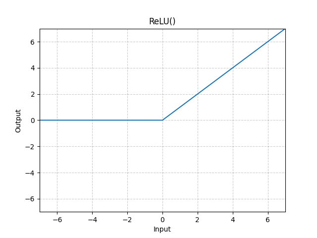
When the input is positive, ReLU can output any value, so it has no upper bound. Why is that a problem? Without an upper bound, we cannot reserve a tightly limited amount of memory for representing the values. ReLU6 addresses this issue and has been evaluated favorably from both fixed-point and training perspectives.

Deep-learning optimization sometimes converts values to fixed point. Setting the upper bound to 6 lets three bits represent all relevant integer levels, which is quite useful for optimization. One analysis also suggests that an upper bound helps a model learn distributed features earlier. The authors reportedly proposed ReLU6 after tests found 6 to be the best-performing bound.

MobileNet V2

Next comes another famous paper, MobileNet V2.

The leftmost block is the MobileNet V1 framework. The center and right blocks are MobileNet V2.

To state the key idea first, MobileNet V2 uses an inverted residual structure. Both V2 blocks begin with pointwise ($1 \times 1$) convolution and ReLU6. The following depthwise convolution uses stride 1 in the left block, preserving the spatial dimensions, and stride 2 in the right block, downsampling them. A final pointwise convolution has no activation function. Downsampling prevents a skip connection because the shapes no longer match, so only the left block has a residual connection.

In more detail, an expansion convolution first increases the number of channels, depthwise convolution processes the result, and pointwise convolution projects it back down. The first $1 \times 1$ convolution expands; the last $1 \times 1$ convolution projects. Omitting an activation after the projection minimizes feature distortion caused by ReLU.

The right side of the figure shows the inverted residual, while the left shows an ordinary residual block. The difference is the expansion in the number of channels. Roughly speaking, the left is the ResNet structure and the right is the structure used in MobileNet V2.

MobileNet V3

Next in the sequence is MobileNet V3.

The paper retains the inverted residual structure. It judged the pointwise and depthwise ideas from MobileNet V1 and the inverted residual from V2 to be useful enough to continue using.

The main differences are a new activation function and the addition of an SE, or Squeeze-and-Excitation, module.

H-Swish

H-swish is a modified swish function. To be honest, I did not know swish very well either, so I looked it up. I hope everyone else says the same.

$$\text{swish}(x) = \frac{x}{1+e^{-x}}$$

It turned out to be just a sigmoid multiplied by $x$—less mysterious than I expected. Since sigmoid itself is not used very often these days, the thought seems to have been: can the modified sigmoid-like swish be expressed with a ReLU-style operation?

And then they did exactly that.

$$\text{h-swish}(x) = x\frac{\text{ReLU6}(x+3)}{6}$$

PyTorch appears to provide it under the name hardswish, for anyone who wants to try it.

SE: Squeeze and Excitation

Squeeze-and-Excitation is already quite famous, and I recommend reading the paper. It is not terribly complicated; the diagram and short explanation are enough to understand the purpose of the module.

Readers of the STN paper may recognize the broad ambition: use a module to optimize attention automatically for each layer. Ordinarily, when using a feature map, we do not explicitly consider which channels contain useful information. SE emerged from the view that this makes learning inefficient.

If pointwise convolution in MobileNet restores cross-channel relationships, a small auxiliary mechanism that reweights channels can have a substantial effect. As the figure shows, the weight calculation is very simple: squeeze the feature map with a spatial average, then pass it through a small function. Very simple indeed.

NAS: Neural Architecture Search

When building a deep network, neither architecture design nor hyperparameter tuning is completely automated. AutoML can be viewed as a process for addressing these design and experience-driven problems.

• Search space: the set of architectures to try
• Search algorithm: how to explore the search space—randomly, through Bayesian optimization, reinforcement learning, and so on
• Evaluation strategy: how the NAS algorithm evaluates candidates, such as ordinary training and validation, full supervision, or few-shot methods

Those are the main terms.

There are many NAS approaches, and spending half a day on them would make the lightweight-model topic feel secondary, so I will stop here. MobileNet V3 optimized its architecture with the NetAdapt algorithm. That probably explains the paper's title: “Searching for MobileNetV3.”